
| 일 | 월 | 화 | 수 | 목 | 금 | 토 |
|---|---|---|---|---|---|---|
| 1 | 2 | 3 | ||||
| 4 | 5 | 6 | 7 | 8 | 9 | 10 |
| 11 | 12 | 13 | 14 | 15 | 16 | 17 |
| 18 | 19 | 20 | 21 | 22 | 23 | 24 |
| 25 | 26 | 27 | 28 | 29 | 30 | 31 |
- deep daiv. project_paper
- deep daiv. week4 팀활동과제
- deep daiv. 2주차 팀 활동 과제
- deep daiv. WIL
- deep daiv. week3 팀활동과제
- Today
- Total
OK ROCK
[NLP] Information Retrieval(2): Keyword-based Retrieval 본문
< Week 3 Contents > 中
1. Keyword-based Retrieval ☜
2. Evaluation Metrics
3. Vector-based Retrieval
1. Keyword-based Retrieval
[ Theory ]
Objective :Query(질의) -> Document(문서)를 찾고자 한다.
(1) Term Frequency := ( tf(t, d) )
단순히 문서(d)에 나타나는 해당 단어(t)의 총 빈도수를 사용하는 것.
즉, 특정 단어가 문서 내에 얼마나 자주 등장하는지를 나타내는 값으로, 이 값이 높을수록 문서에서 중요하다고 생각할 수 있다.
문서 d 내에서 단어 t의 총 빈도를 f(t,d)라 할 경우, 가장 간단한 방법은 tf(t, d) = f(t, d)로 구할 수 있지만, 그 외에 다음과 같은 방식들로 TF값을 산출할 수 있다.
- Boolean 빈도: tf(t,d) = t가 d에 한 번이라도 나타나면 1, 아니면 0;
- Log scale 빈도: tf(t,d) = log (f(t,d) + 1);
- 증가 빈도: 최빈 단어를 분모로 target 단어의 TF를 나눈 값으로, 일반적으로는 문서의 길이가 상대적으로 길 경우, 단어 빈도값을 조절하기 위해 사용한다.

↔ 하지만 단어 자체가 문서군(문서집합, D) 내에서 자주 사용되는 경우, 이것은 그 단어가 전체 문서에서 흔하게 등장한다는 것을 의미하고, 이것을 DF(문서 빈도, document frequency)라고 따로 떼어내서 생각할 수 있다. .DF의 역수를 IDF라고 생각할 수 있고, (2)에 바로 등장하니 살펴보도록 하자.
(2) Inverse Document Frequency :=( idf(t, D) )
한 단어가 문서 집합 전체에서 얼마나 공통적으로 나타나는지를 나타내는 값.
전체 문서의 수를 해당 단어를 포함한 문서의 수로 나눈 뒤 로그를 취하여 얻을 수 있다.

- |D| : 문서 집합 D의 크기, 또는 전체 문서의 수
- | {d ∈ D, t ∈ d }| : 단어 t가 포함된 문서의 수.(즉, Document Frequency). 단어가 전체 말뭉치(corpus) 안에 존재하지 않을 경우 이는 분모가 0이 되는 결과를 가져온다. 이를 방지하기 위해 1+| {d ∈ D, t ∈ d } |로 쓰는 것이 일반적이다.
↔ idf(t, D)값이 클수록, 전체 문서 집합(D) 내에서 그 특정 단어가 드물게 등장하는 것으로 해석할 수 있다.
(3) TF- IDF(term frequency - inverse document freuqency)
위에서 구한 TF와 IDF를 곱한 값을 의미한다.

↔ 특정 문서 내에서 단어 빈도가 높을 수록, 그리고 전체 문서들 중 그 단어를 포함한 문서가 적을 수록 TF-IDF값이 높아진다. 따라서 이 값을 이용하면 모든 문서에 흔하게 나타나는 단어를 걸러내는 효과를 얻을 수 있다.
↔ IDF의 로그 함수 안의 값은 항상 1 이상이므로, IDF값과 TF-IDF값은 항상 0 이상이 된다. 특정 단어를 포함하는 문서들이 많을 수록 로그 함수 안의 값이 1에 가까워지게 되고, 이 경우 IDF값과 TF-IDF값은 0에 가까워지게 된다.
[ Code Review ]
data 불러오는 과정과 같은 개인적으로 중요하지 않다고 생각하는 부분은 cut하였습니다.
# 1. Term Frequency(TF)
|
1
2
3
4
5
6
7
8
9
10
11
12
13
|
n_docs = 90 #|D| = 90으로 설정
import konlpy
tokenizer_engine = konlpy.tag.Okt()
tokenizer = tokenizer_engine.morphs #토크나이저 불러옵니다.
from sklearn.feature_extractin.text import CountVectorizer #Term-Frequency 계산해주는 역할
vec = CountVectorizer(tokenizer = tokenizer, max_features = 100)
X = vec.fit_transform([x["precedent"] for x in docs]) df = pd.DataFrame(X.toarray(), columns = vec.get_features_names_out()) df
# df 출력 결과, term-frequency가 아래와 같이 나타납니다.
|
cs |

# 2. Inverted Index(IDF)
|
1
2
3
4
5
6
7
8
9
10
11
12
13
14
15
16
17
18
19
20
21
|
from collections import defaultdict
from tqdm import tqdm #진행속도 시각화하기위한 용도
inverted_doc_indexes = defaultdict(dict)
#어떤 단어(word)가, 어떤 id의 문서에서(doc-id), 어떤 위치(word-location)에 존재하는지 출력할 dict
docs_with_tokens = {}
doc_ids = [x["ids"] for x in docs]
for doc in tqdm(docs):
toks = tokenizer(doc["precedent"])
doc_id = doc["id"]
docs_with_tokens[doc_id] = toks
tok2tok_location = defaultdict(list) # 특정문서에서 토큰들이 어디 위치에 있는지 출력
for i_tok, tok in enumerate(toks):
tok2tok_location[tok].append(i_tok)
for tok, tok_locations in tok2tok_location.items():
inverted_doc_indexes[tok][doc_id] = tok_locations # word / doc-id / word-location
|
cs |
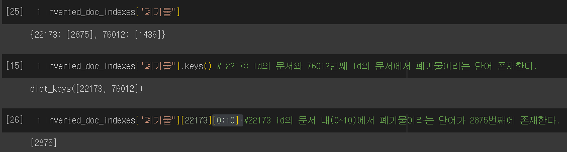
출력 예시)
# 3. Running Boolean Search using IDF
|
1
2
3
4
5
6
7
8
9
10
11
12
13
14
15
16
|
from functools import reduce
def boolean_search(query, inverted_doc_indexes, doc_ids, tokenizer):
toks = tokenizer(query)
doc_ids_with_tok = [set(inverted_doc_indexes[tok].keys()) for tok in toks]
# token이 위치한 문서의 세트를 전부 가져옴
doc_ids = reduce(lambda x, y : x.intersection(y), doc_ids_with_tok, set(doc_ids))
# 두 개의 단어 모두 존재하는 교집합 문서들을 찾아옴
return doc_ids
#(ex)
boolean_search("피고인을 징역", inverted_doc_indexes, doc_ids, tokenizer)
# 결과 = {3161, 50345, 50473, 62312, 72446, 73032, 78368, 84858, ....}
|
cs |
# 3.TF-IDF
위에서 구한 inverted_doc_indexes 딕셔너리를 활용해서, doc-frequency를 다음과 같이 구할 수 있습니다.
(전체 문서집합에서 특정 단어가 몇 번 존재하는지)
|
1
2
3
4
5
6
7
8
9
|
doc_freq = {}
for word in inverted_doc_indexes.keys():
doc_freq[word] = len(inverted_doc_indexes[word].keys()]
{x: doc_freq[x] for x in sorted(doc_freq, key = lambda x : doc_freq[x], reverse = True)}
# 출력결과: {'주문' : 90, '\n': 90, '에':90, '한다': 90, '.': 90, '이유': 90, .....}
# 해석 = 주문이라는 단어 90개의 문서 집합에서 90번 모두 존재한다는 의미
|
cs |
가장 핵심이 되는 코드가 아래에 있습니다.@@!!★집중

|
1
2
3
4
5
6
7
8
9
10
11
12
13
14
15
|
tf_idf = {}
for doc_id in tqdm(doc_ids):
for tok in docs_with_tokens[doc_id]:
tf = len(inverted_doc_indexes[tok][doc_id] #term-frequency
# tf = (1+np.log(tf) if tf >0 else 0)
if tok in doc_freq:
df = doc_freq[tok] # document-freqency
else:
df = 0
idf = np.log((len(doc_ids} +1 ) / (df+1)) # inverse-df
tf_idf[(doc_id, tok)] = tf*idf # Finally tf-idf !
|
cs |
tf_idf : doc_id / token / score저장되어있음
# 마지막으로, 구현한 tf-idf를 이용해서 Ranked_search를 run해봅시다
|
1
2
3
4
5
6
7
8
9
10
11
12
13
14
15
16
17
18
19
20
|
def ranked_search(query, tokenizer, k, tf_idf_index, doc_ids):
words = tokenzier(query)
scores = []
for doc_id in doc_ids:
score = 0
for word in words:
if (doc_id, word) in tf_idf_index:
score += tf_idf_index[(doc_id, word)]
scores.append((doc_id, score))
scores_trimmed = sorted(scores, key = lambda x : x[-1], reverse = True)[0:k]
return scores_trimmed
# (ex)
ranked_search("사기 사건 비트코인", tokenizer, 10, tf_idf, doc_ids)
# query가 들어있는 문서들의 score(tf_idf값)이 어떻게 변해가는지 과정 확인 가능 |
cs |
Reference
'Study > NLP' 카테고리의 다른 글
| [NLP] Text Generation(1) : Decoding (0) | 2023.10.13 |
|---|---|
| [NLP] Information Retrieval(3): Vector-based Retrieval (0) | 2023.09.30 |
| [NLP] Information Retrieval(1): Evaluation Metrics (0) | 2023.09.27 |
| [NLP] Byte-Pair Encoding tokenization (5) | 2023.09.17 |


